The relationship between class/income and cars
As a passionate cyclist in Vienna, I often find myself in dangerous situations with cars (mostly SUVs) in Vienna. Even though the cycling infrastructure is improving, the traffic is very dense. As a person that is concerned by climate change and social justice I would love to see the city change to a greener, car reduced one with good cycling infrastructure.
There is empiric evidence, that higher wealth and income is correlated with a higher CO2 footprint. Individual car traffic is one source of CO2 and we can assume, that higher wealth correlates with more cars and also heavier, more powerful cars. During my data-science-in-Python-learning-journey, I investigated this relationship with aggregated data from different districts of Vienna, Austria and wanted to know:
How is average net income related to the amount of cars per capita (and the type of car in terms of power) in the districts of Vienna?
Let’s see.
Data & Method
I grabed some data from https://www.data.gv.at/ published by the city of Vienna. The datasets contain different variables per district and year, spanning the years from 2001-2022. I merged the following datasets (see source code from Jupyter Notebook below or check out the notebook on my Github Repository):
- Car density in Vienna: https://www.data.gv.at/katalog/dataset/72e189ed-e418-4353-9838-70301e3ca12c
- Source CSV: https://www.wien.gv.at/gogv/l9ogdpkwdichte2022
- Cars categorized by power in Vienna: https://www.data.gv.at/katalog/dataset/3828fd26-5284-444b-ba25-a68a84e91bd
- Average net income per district in Vienna: https://www.data.gv.at/katalog/dataset/d76c0e8b-c599-4700-8a88-29d0d87e563d
I calculated correlation coefficients (Pearson & Spearman) for average income & car density (grouped by district & year and per district for the total period with the yearly values aggregated by mean). I also calculated a ratio for heavy power cars vs. low power cars per district by dividing the sum of cars with more or equal than 131 KW power by the sum of cars with less than 131 KW power. I then visualized the relationship between average income and car density per district with aggregated values, adding the power ratio variable as a third variable to visualize the size of the drawn points.
Results
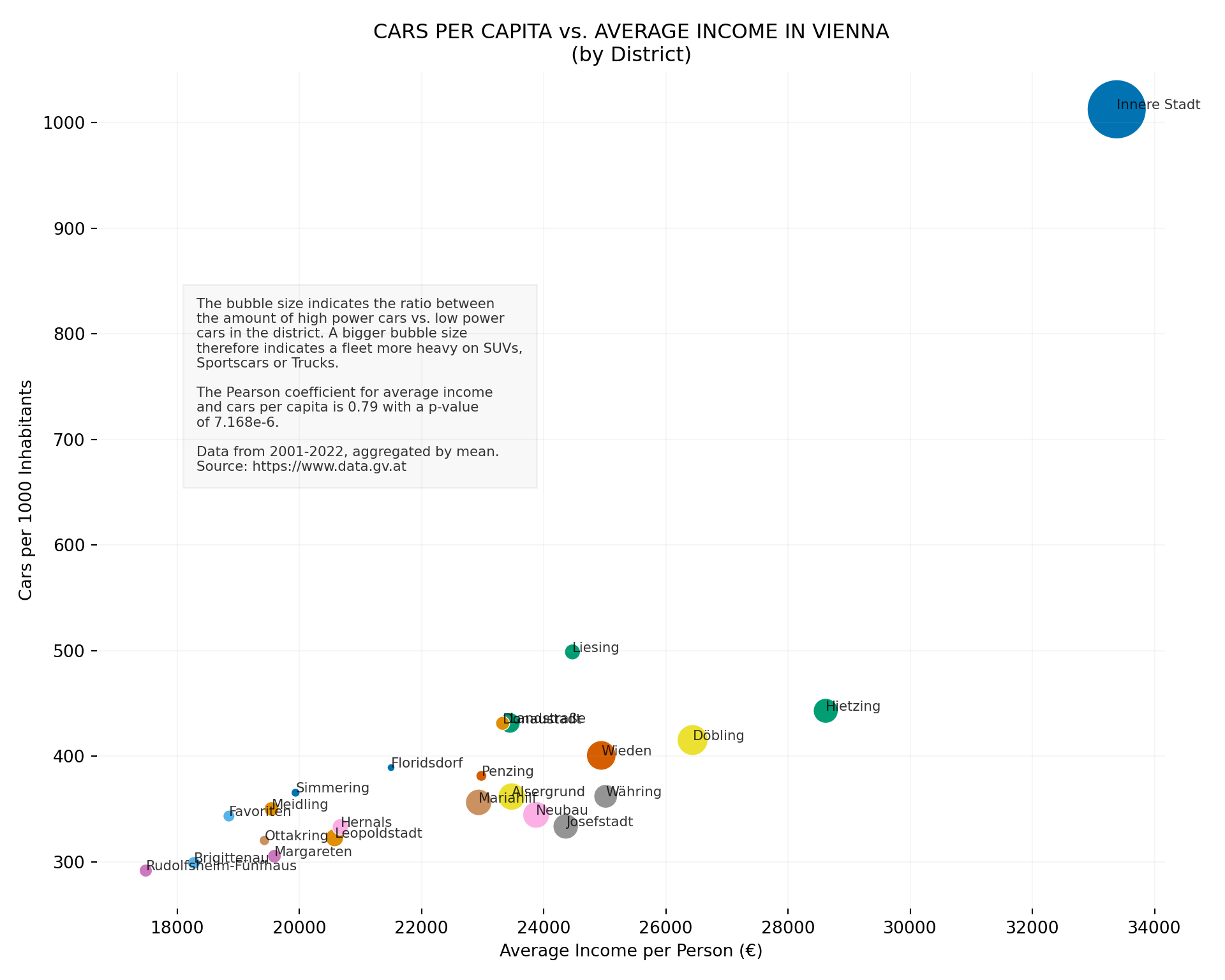
I find very clear correlations between the average income in districts and the amount of cars per capita per district.1 More so, in high income districts the ratio of cars with more horsepower vs. cars with less horsepower is higher than in low income districts. Very striking is the first district: it deviates strongly from the others in terms of income, car per capita and car power ratio:
The data suggests an overall stratification by class/income. In the typical working-class districts of Floridsdorf, Favoriten, Brigittenau, Margareten and Ottakring, both income and car ownership per 1000 inhabitants are low. In addition, the number of high-performance (and therefore particularly high-emission) cars is relatively low there (see bubblesize of the districts). In the middle-class districts adjacent to the first district within the “Gürtel”, incomes are higher in average and the density of cars and SUVs is also increasing. In the richer, middle-class districts of Döbling and Hietzing, the average income is indeed higher and with it the number of cars, which are proportionately more powerful (i.e. SUVs etc.).
The first district is very striking: it deviates significantly from the other districts in all three dimensions. I found this quite astonishing, I would not have expected such a big difference to districts like Döbling. The first district of Vienna is the historic main town, which was surrounded by city walls, home to all the great buildings from the era of the Habsburg monarchy and today is still the center of power. While in the other districts there is 1 car per 2 or 3 people, there is a car for every person living in the first district. However, this distinct features may also be due to the fact that in all districts except the first, the social mix is higher due to communal social housing. There might be other reasons, that I am not aware of. There almost have to be some, as the difference is so extreme.
The government in Vienna is very cautious when it comes to policies such as road pricing in inner districts or higher taxes on SUVs. The results suggest that this may also have to do with the wealthy clientele (including SPÖ party members?) in the first district, who would be snubbed.
In sum, this is another example of why the goal of mitigating and adapting to climate change also needs to address the social question of economic inequality.
Source code
If you want to run the code yourself, checkout this Jupyter notebook.
Loading and preparing the data
import pandas as pd
import matplotlib.pyplot as plt
import numpy as np
import seaborn as sns
from scipy.stats import pearsonr
from scipy.stats import spearmanr

import warnings
warnings.filterwarnings('ignore')
Load data: Cars per district
# Source: https://www.data.gv.at/katalog/dataset/72e189ed-e418-4353-9838-70301e3ca12c#additional-info
pkwdichte22 = pd.read_csv('https://www.wien.gv.at/gogv/l9ogdpkwdichte2022', decimal=",", sep=";")
del(pkwdichte22['NUTS1'])
del(pkwdichte22['NUTS2'])
del(pkwdichte22['NUTS3'])
del(pkwdichte22['SUB_DISTRICT_CODE'])
del(pkwdichte22['REF_YEAR'])

pkwdichte22["YEAR"] = pd.to_datetime(pkwdichte22["YEAR"], format='%Y')

pkwdichte22["DISTRICT_CODE"][pkwdichte22["DISTRICT_CODE"] == 9] = pkwdichte22["DISTRICT_CODE"] + 89992
pkwdichte22["DISTRICT_CODE"] = ((pkwdichte22["DISTRICT_CODE"] - 90001)/100).astype(int)
pkwdichte22['CARS_PER_1000_CAPITA'] = pkwdichte22['CARS_PER_1000_CAPITA'].str.replace(",",".",regex=False).str.replace(" ", "", regex=False).astype(float)
Load data: Cars categorized by power (KW) since 2011
# Source: https://www.data.gv.at/katalog/dataset/3828fd26-5284-444b-ba25-a68a84e91bdf#additional-info
pkwleistung = pd.read_csv('https://www.wien.gv.at/gogv/l9ogdviebeztecsexvehkw2011f', sep=";", header=1)
del(pkwleistung['NUTS'])
del(pkwleistung['SUB_DISTRICT_CODE'])
del(pkwleistung['REF_DATE'])

pkwleistung["REF_YEAR"] = pd.to_datetime(pkwleistung["REF_YEAR"], format='%Y')
pkwleistung.rename({'REF_YEAR': 'YEAR'}, axis=1, inplace=True)

pkwleistung["DISTRICT_CODE"] = ((pkwleistung["DISTRICT_CODE"] - 90000)/100).astype(int)

pkwleistung = pkwleistung[pkwleistung['DISTRICT_CODE'] < 24]

pkwleistung = pkwleistung.groupby(['DISTRICT_CODE', 'YEAR'], as_index=False).sum(numeric_only=True)
del(pkwleistung['SEX'])

pkwleistungwien = pkwleistung.groupby(['YEAR'], as_index=False).sum(numeric_only=True)
pkwleistungwien['DISTRICT_CODE'] = 0
pkwleistung = pd.concat([pkwleistung, pkwleistungwien])
Load data: Average net income by district
# Source: https://www.data.gv.at/katalog/dataset/d76c0e8b-c599-4700-8a88-29d0d87e563d#resources
inc = pd.read_csv('https://www.wien.gv.at/gogv/l9ogdviebezbizecnincsex2002f', sep=";", header=1, thousands=".")

del(inc['NUTS'])
del(inc['SUB_DISTRICT_CODE'])
del(inc['REF_DATE'])

inc["REF_YEAR"] = pd.to_datetime(inc["REF_YEAR"], format='%Y')
inc.rename({'REF_YEAR': 'YEAR'}, axis=1, inplace=True)

inc["DISTRICT_CODE"] = ((inc["DISTRICT_CODE"] - 90000)/100).astype(int)
inc = inc.iloc[:, :5]
Merge the datasets
df = (pd.merge(pkwdichte22, pkwleistung, how="left", on=['DISTRICT_CODE', "YEAR"])
        .merge(inc, how="left", on=['DISTRICT_CODE', "YEAR"])
)
#df = df[(df["YEAR"].dt.year < 2023) & (df["YEAR"].dt.year > 2001)]
df.head()
##    DISTRICT_CODE       YEAR  ... INC_MAL_VALUE  INC_FEM_VALUE
## 0              0 2001-01-01  ...           NaN            NaN
## 1              0 2002-01-01  ...       20709.0        15424.0
## 2              0 2003-01-01  ...       20845.0        15526.0
## 3              0 2004-01-01  ...       21033.0        15684.0
## 4              0 2005-01-01  ...       21503.0        16137.0
##
## [5 rows x 15 columns]
df.info()
## <class 'pandas.core.frame.DataFrame'>
## RangeIndex: 390 entries, 0 to 389
## Data columns (total 15 columns):
##  #   Column                Non-Null Count  Dtype
## ---  ------                --------------  -----
##  0   DISTRICT_CODE         390 non-null    int64
##  1   YEAR                  390 non-null    datetime64[ns]
##  2   DISTRICT              390 non-null    object
##  3   CARS_PER_1000_CAPITA  390 non-null    float64
##  4   KW_0_30               288 non-null    float64
##  5   KW_31_50              288 non-null    float64
##  6   KW_51_70              288 non-null    float64
##  7   KW_71_90              288 non-null    float64
##  8   KW_91_110             288 non-null    float64
##  9   KW_111_130            288 non-null    float64
##  10  KW_131_150            288 non-null    float64
##  11  KW_151_+              288 non-null    float64
##  12  INC_TOT_VALUE         365 non-null    float64
##  13  INC_MAL_VALUE         365 non-null    float64
##  14  INC_FEM_VALUE         365 non-null    float64
## dtypes: datetime64[ns](1), float64(12), int64(1), object(1)
## memory usage: 45.8+ KB
Prepare the data for bivariate analysis (Income and Cars per Capita)
inccarsgrp = df[(df['DISTRICT_CODE']>0)&(df['INC_TOT_VALUE']>0)].groupby('DISTRICT_CODE').agg({'DISTRICT': 'first',
                                                   'INC_TOT_VALUE': np.mean,
                                                   'KW_0_30': np.mean,
                                                   'KW_31_50': np.mean,
                                                   'KW_51_70': np.mean,
                                                   'KW_71_90': np.mean,
                                                   'KW_91_110': np.mean,
                                                   'KW_111_130': np.mean,
                                                   'KW_131_150': np.mean,
                                                   'KW_151_+': np.mean,
                                                   'CARS_PER_1000_CAPITA': np.mean
                                                   })
inccarsgrp['DISTRICT'] = inccarsgrp['DISTRICT'].replace("^Wien\s", "", regex=True)
# Define powerful and less powerful cars
inccarsgrp['powerful_cars'] = inccarsgrp[['KW_131_150', 'KW_151_+']].sum(axis=1)
inccarsgrp['less_powerful_cars'] = inccarsgrp[['KW_0_30', 'KW_31_50', 'KW_51_70', 'KW_71_90', 'KW_91_110','KW_111_130']].sum(axis=1)

# Avoid divide-by-zero
inccarsgrp['POWER_RATIO'] = inccarsgrp['powerful_cars'] / (inccarsgrp['less_powerful_cars'] + 1e-9)  # Add small number to avoid divide by zero

# Create power_ratio bins (5 quantiles)
inccarsgrp['CARPOWER_RATIO'] = pd.qcut(inccarsgrp['POWER_RATIO'], q=5, labels=[
    'Very Low', 'Low', 'Medium', 'High', 'Very High'
])
# Reverse the size mapping
size_mapping = {
    'Very Low': 100,
    'Low': 200,
    'Medium': 400,
    'High': 600,
    'Very High': 800
}

# Apply the mapping
inccarsgrp['CARPOWER_RATIO'] = inccarsgrp['CARPOWER_RATIO'].map(size_mapping)
Check Correlations
All districts
# Check for ungrouped data
df_dist = df[(df['DISTRICT_CODE']>0)&(df['INC_TOT_VALUE']>0)].dropna() # Only keep district data and remove summary data for whole Vienna
print(len(df_dist))
## 253
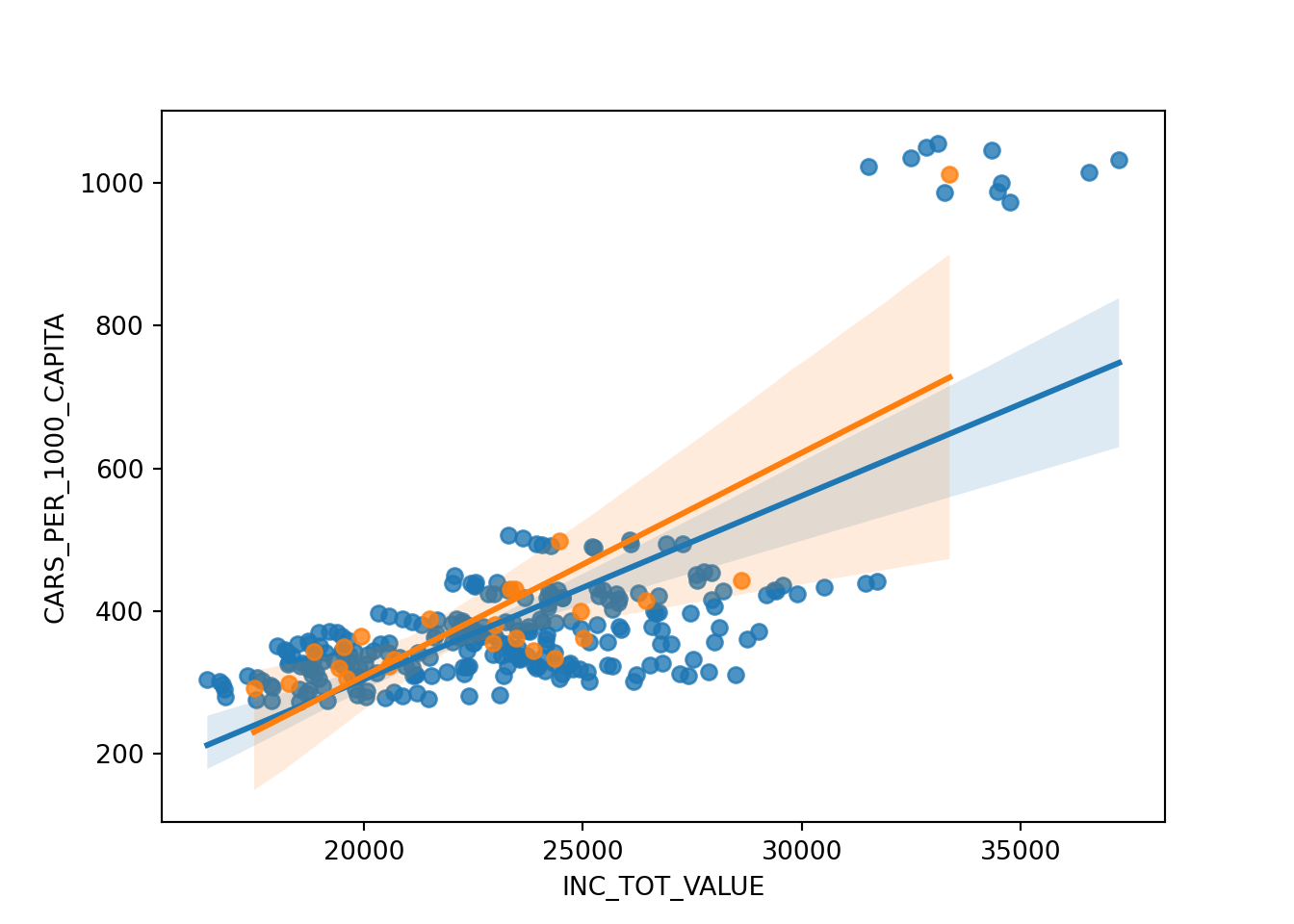
corr, p_value = pearsonr(df_dist['INC_TOT_VALUE'], df_dist['CARS_PER_1000_CAPITA'])
print(f"Pearson correlation: {corr:.2f}, p-value: {p_value:.40f}")
## Pearson correlation: 0.70, p-value: 0.0000000000000000000000000000000000000113
corr_s, p_s = spearmanr(df_dist['INC_TOT_VALUE'], df_dist['CARS_PER_1000_CAPITA'])
print(f"Spearman correlation: {corr_s:.2f}, p-value: {p_s:.30f}")
## Spearman correlation: 0.59, p-value: 0.000000000000000000000000919457
sns.regplot(data=df_dist, x="INC_TOT_VALUE", y="CARS_PER_1000_CAPITA")

# Check for yearly grouped aggregates
corr, p_value = pearsonr(inccarsgrp['INC_TOT_VALUE'], inccarsgrp['CARS_PER_1000_CAPITA'])
print(f"Pearson correlation: {corr:.2f}, p-value: {p_value:.9f}")
## Pearson correlation: 0.79, p-value: 0.000007168
corr_s, p_s = spearmanr(inccarsgrp['INC_TOT_VALUE'], inccarsgrp['CARS_PER_1000_CAPITA'])
print(f"Spearman correlation: {corr_s:.2f}, p-value: {p_s:.9f}")
## Spearman correlation: 0.76, p-value: 0.000023099
sns.regplot(data=inccarsgrp, x="INC_TOT_VALUE", y="CARS_PER_1000_CAPITA")
Excluding the first district (outlier)
# Check for ungrouped data
df_dist = df[(df['DISTRICT_CODE']>1)&(df['INC_TOT_VALUE']>0)].dropna() # Only keep district data and remove summary data for whole Vienna
print(len(df_dist))
## 242
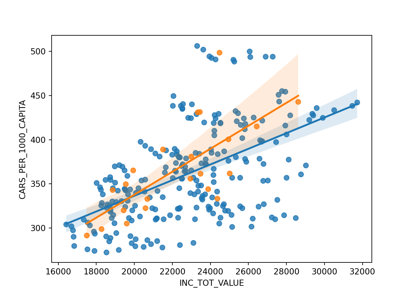
corr, p_value = pearsonr(df_dist['INC_TOT_VALUE'], df_dist['CARS_PER_1000_CAPITA'])
print(f"Pearson correlation: {corr:.2f}, p-value: {p_value:.20f}")
## Pearson correlation: 0.53, p-value: 0.00000000000000000034
corr_s, p_s = spearmanr(df_dist['INC_TOT_VALUE'], df_dist['CARS_PER_1000_CAPITA'])
print(f"Spearman correlation: {corr_s:.2f}, p-value: {p_s:.20f}")
## Spearman correlation: 0.53, p-value: 0.00000000000000000097
sns.regplot(data=df_dist, x="INC_TOT_VALUE", y="CARS_PER_1000_CAPITA")

# Check for yearly grouped aggregates
corr, p_value = pearsonr(inccarsgrp[inccarsgrp['DISTRICT']!="Innere Stadt"]['INC_TOT_VALUE'], inccarsgrp[inccarsgrp['DISTRICT']!="Innere Stadt"]['CARS_PER_1000_CAPITA'])
print(f"Pearson correlation: {corr:.2f}, p-value: {p_value:.9f}")
## Pearson correlation: 0.71, p-value: 0.000192311
corr_s, p_s = spearmanr(inccarsgrp[inccarsgrp['DISTRICT']!="Innere Stadt"]['INC_TOT_VALUE'], inccarsgrp[inccarsgrp['DISTRICT']!="Innere Stadt"]['CARS_PER_1000_CAPITA'])
print(f"Spearman correlation: {corr_s:.2f}, p-value: {p_s:.9f}")
## Spearman correlation: 0.73, p-value: 0.000118941
sns.regplot(data=inccarsgrp[inccarsgrp['DISTRICT']!="Innere Stadt"], x="INC_TOT_VALUE", y="CARS_PER_1000_CAPITA")
Visualization
plt.figure(figsize=(10,8))
palette = sns.color_palette("colorblind")
plt.grid(alpha=0.1)

# Create scatterplot with 3 dimensions for every district
scatter = sns.scatterplot(
    data=inccarsgrp,
    x='INC_TOT_VALUE',
    y='CARS_PER_1000_CAPITA',
    size='POWER_RATIO',         # Size = how SUV-heavy is the fleet?
    hue='DISTRICT',
    palette=palette,
    sizes=(20, 1200),
    legend=False
)

# Iterate over districts, create text labels
for _, row in inccarsgrp.iterrows():
    plt.text(
        row['INC_TOT_VALUE'],
        row['CARS_PER_1000_CAPITA'],
        row['DISTRICT'],
        fontsize=8,
        alpha=0.8,
    )
## Text(33380.86666666667, 1012.5486666666667, 'Innere Stadt')
## Text(20577.333333333332, 322.7033333333333, 'Leopoldstadt')
## Text(23446.6, 431.386, 'Landstraße')
## Text(24942.4, 400.63, 'Wieden')
## Text(19591.866666666665, 305.152, 'Margareten')
## Text(22936.0, 356.17133333333334, 'Mariahilf')
## Text(23876.466666666667, 344.32866666666666, 'Neubau')
## Text(24360.8, 333.3933333333333, 'Josefstadt')
## Text(23477.4, 361.6526666666667, 'Alsergrund')
## Text(18847.6, 343.17199999999997, 'Favoriten')
## Text(19937.866666666665, 365.316, 'Simmering')
## Text(19543.6, 349.9053333333333, 'Meidling')
## Text(28617.333333333332, 442.8846666666667, 'Hietzing')
## Text(22980.066666666666, 381.26599999999996, 'Penzing')
## Text(17486.666666666668, 291.586, 'Rudolfsheim-Fünfhaus')
## Text(19428.866666666665, 320.11800000000005, 'Ottakring')
## Text(20671.866666666665, 332.94533333333334, 'Hernals')
## Text(25014.733333333334, 361.9166666666667, 'Währing')
## Text(26437.8, 415.1806666666667, 'Döbling')
## Text(18274.933333333334, 298.8726666666667, 'Brigittenau')
## Text(21501.6, 389.05, 'Floridsdorf')
## Text(23328.6, 431.03266666666667, 'Donaustadt')
## Text(24471.133333333335, 498.6273333333333, 'Liesing')
ax = plt.gca()
ax.text(18320,
         670,
"""The bubble size indicates the ratio between\nthe amount of high power cars vs. low power
cars in the district. A bigger bubble size\ntherefore indicates a fleet more heavy on SUVs,
Sportscars or Trucks.\n
The Pearson coefficient for average income
and cars per capita is 0.79 with a p-value
of 7.168e-6.\n
Data from 2001-2022, aggregated by mean.\nSource: https://www.data.gv.at""",
         fontsize=8,
         alpha=0.8,
         bbox=dict(boxstyle="square,pad=1", facecolor='gray', alpha=0.05)
)
## Text(18320, 670, 'The bubble size indicates the ratio between\nthe amount of high power cars vs. low power\ncars in the district. A bigger bubble size\ntherefore indicates a fleet more heavy on SUVs,\nSportscars or Trucks.\n\nThe Pearson coefficient for average income\nand cars per capita is 0.79 with a p-value \nof 7.168e-6.\n\nData from 2001-2022, aggregated by mean.\nSource: https://www.data.gv.at')
# remove the frame of the chart
for spine in plt.gca().spines.values():
    spine.set_visible(False)

plt.title('CARS PER CAPITA vs. AVERAGE INCOME IN VIENNA\n(by District)')
## Text(0.5, 1.0, 'CARS PER CAPITA vs. AVERAGE INCOME IN VIENNA\n(by District)')
plt.xlabel('Average Income per Person (€)')
## Text(0.5, 0, 'Average Income per Person (€)')
plt.ylabel('Cars per 1000 Inhabitants')
## Text(0, 0.5, 'Cars per 1000 Inhabitants')
plt.tight_layout()
plt.show()
Excursus: Reference data for categorizing cars by power
# Get some references for power categories
cars = pd.read_csv('https://raw.githubusercontent.com/CikuKariuki/Cars/refs/heads/master/Cars%20Data.csv')
cars['KW'] = cars['Horsepower'] / 0.73549875 # Convert horsepower to KW
carsg = cars.groupby('Type').agg({"KW":np.mean}).sort_values('KW', ascending=False)
carsg
##                 KW
## Type
## Sports  386.354518
## SUV     320.621438
## Truck   305.688260
## Sedan   274.176521
## Wagon   263.766594
## Hybrid  125.085189
The Pearson coefficient for average income and cars per capita aggregated by mean for all years (2001-2022) on a district level is 0.79 with a p-value of 0.000007168. The Spearman correlation is 0.76, with a p-value of 0.000023099. ↩︎